
| Creating plots with the Data Wizard |
| Prev | The Kst Tutorial | Next |
Kst can also be completely controlled through the graphical user interface,
without ever using the command line. In this section, we will look at
the Data Wizard, which a quick and easy way of creating vectors,
curves, and plots in Kst from data files. To launch the wizard,
select from the
menu or click the
![]() button on the toolbar. You will be prompted to select a data source by the
following dialog:
button on the toolbar. You will be prompted to select a data source by the
following dialog:

Select the gyrodata.dat file used in the
command-line examples. If you have completed the command-line exercises
in the previous sections, then the file should be listed in the recent
files list, as shown. Simply click on it to select it. Otherwise,
enter the full path in the top text entry box (or click on the
![]() icon and browse to the file). Once you have selected the file, the
button will be enabled. Click on it to proceed to the next page.
The following window will be displayed:
icon and browse to the file). Once you have selected the file, the
button will be enabled. Click on it to proceed to the next page.
The following window will be displayed:
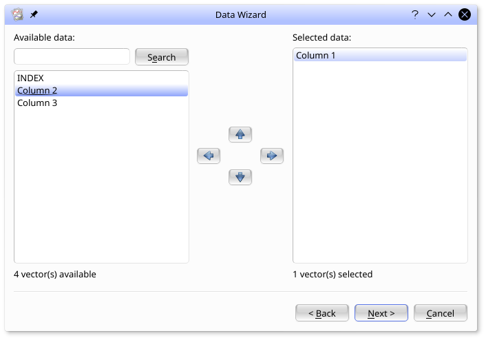
Fields in gyrodata.dat available to be plotted are
listed in the Available data box on the left. Fields
that have been selected for plotting are listed in the Selected data
box on the right. In the image shown, Column 1 has been
selected for plotting.
Select Column 1, Column 2, and Column 3 for plotting by moving them to the Selected data box.
To move a field from Available data to
Selected data, double click on it, or
highlight it (with mouse or keyboard) and click on the
![]() icon. As well as using the mouse or keyboard, you may highlight fields by
entering a string to match into the text box above the list. Wildcards such as
icon. As well as using the mouse or keyboard, you may highlight fields by
entering a string to match into the text box above the list. Wildcards such as *,
? and [ ] are
supported.
Click once you have selected the three columns of data.
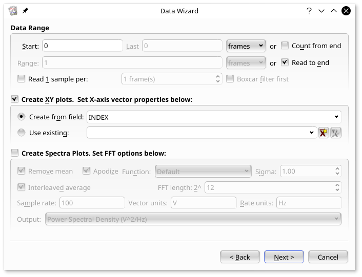
The next tab is used to select the data range to be plotted, and whether to create XY plots, spectrum plots, or both.
The Data Range section is used to specify the
range of data to read from the selected vectors in the input file. The
following discussion assumes knowledge of “frames”. For ASCII
files such as gyrodata.dat, a frame is simply a row of
data, though for other formats this can be more complicated.
Using these five settings, the lower and upper boundaries of the data range can be set. The settings in the above image are set to read the entire data file (starting at frame 0, and reading to the end).
If new data were being appended to the end of the file in real time, then the range would be continuously increasing and Kst would update to reflect this. If instead one wanted to only display the last 1000 frames of the file, one would instead select Count from end and enter 1000 in Range. Kst would scroll the data along as new data were appended to the data file.
The number of data points plotted can be reduced using this option. If Read 1 sample per N frames is not selected, all samples in the selected range will be read. Alternatively, frames in the data file can be skipped by selecting Read 1 sample per N frames. For now, read all of the data by deselecting Read 1 sample per N frames, as shown.
In this tutorial, we are only going to plot the gyroscope time series, and not spectra. To do this, select Create XY plots and deselect Create Spectra Plots as shown.
Set the X axis vectors for the curves to be The vector to be INDEX by selecting Create from field and selecting INDEX in vector selector, as shown.
The FFT Options subsection in the Plot Types section is available only if a power spectrum is to be plotted. This tutorial will not deal with the details of power spectra.
Once you are satisfied with all the settings, click to advance to the next window.
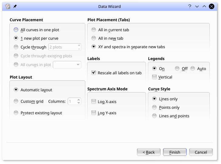
From here, you can change general plotting settings. Most of the settings are self-explanatory. Select 1 new plot per curve for Curve Placement.
Once you are satisfied with all the settings, click and the plots will be generated:
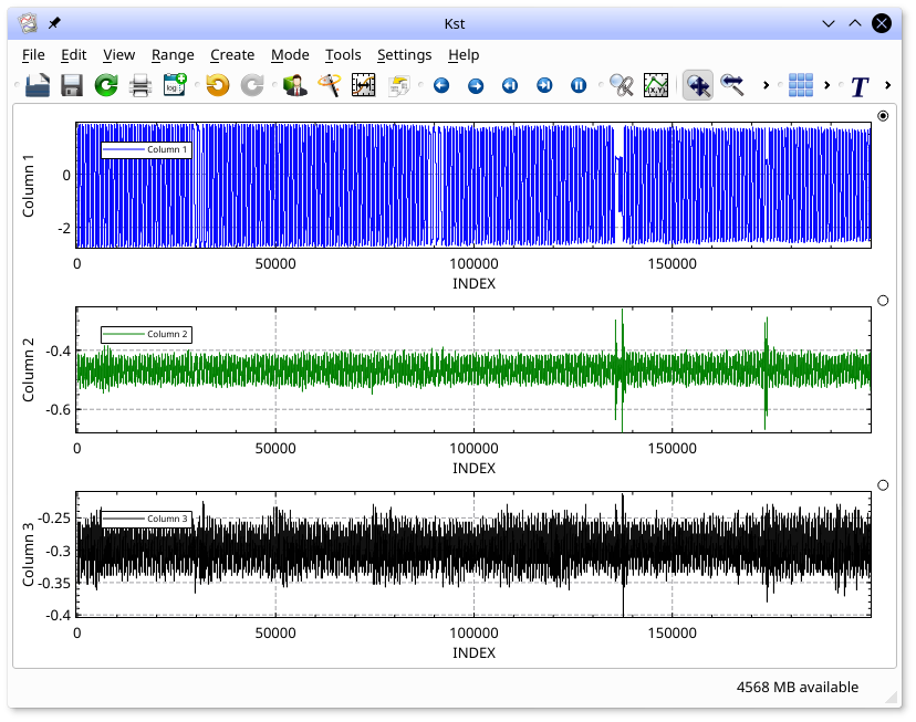
Generating these plots took a bit of effort, so we should save the
current Kst session (it will be used in the next section of this
tutorial). Select from the
menu, and save the session as
mykstsession.kst:
Saving a Kst session saves all the plots, data objects (you will learn about these later), and layouts that exist at the time of saving.
Once the file has been saved, you can exit Kst.
| Prev | Contents | Next |
| Creating plots from the Command-line | Up | The Basics of Plot Manipulation |