
| Creating plots from the Command-line |
| Prev | The Kst Tutorial | Next |
A common use of Kst is to quickly produce plots of data from the command-line. This method of producing plots requires almost no knowledge of Kst's graphical user interface, yet produces immediate, useful results.
The following instructions assume you are working in a broadly bash-compatible shell, such as you would in linux or MacOS.
To obtain an overview of all available Kst command-line options, type:
kst2 --help
A syntax description and list of commands similar to the following will be displayed:
KST Command Line Usage
************************
*** Load a kst file: ***
kst [OPTIONS] kstfile

[OPTIONS] will override the datasource parameters for all data sources in the kst file:
      -F  <datasource>
      -f  <startframe>
      -n  <numframes>
      -s  <frames per sample>
      -a                       (apply averaging filter: requires -s)

************************
*** Read a data file ***
kst datasource OPTIONS [datasource OPTIONS []]

OPTIONS are read and interpreted in order. Except for data object options, all are applied to all future data objects, unless later overridden.
Output Options:
      --print <filename>       Print to file and exit.
      --landscape              Print in landscape mode.
      --portrait               Print in portrait mode.
      --Letter                 Print to Letter sized paper.
      --A4                     Print to A4 sized paper.
      --png <filename>         Render to a png image, and exit.
      --pngHeight <height>     Height of png image (pixels)
      --pngWidth <width>       Width of png image (pixels)
File Options:
      -f <startframe>          default: 'end' counts from end.
      -n <numframes>           default: 'end' reads to end of file
      -s <frames per sample>   default: 0 (read every sample)
      -a                       apply averaging filter: requires -s

Ascii File Options - for ascii files only: these are all sticky
      --asciiDataStart <Line>  Data starts here. Files start at line 1.
      --asciiFieldNames <Line> Field names are in this row.
      --asciiNoFieldNames      Fields are named for their data column
      --asciiReadUnits <Line>  Read units from line <Line>
      --asciiNoUnits           Do not read units
      --asciiSpaceDelim        Columns are Space/tab delimited
      --asciiDelim <char>      Columns are delimited with <char>
      --asciiFixedWidth <w>    Columns have width <w>
      --asciiNoFixedWidth      Columns are delimited, not fixed width
      --asciiDecimalDot        Use a . as a decimal separator (ie, 10.1)
      --asciiDecimalComma      Use a , as a decimal separator (ie, 10,1)
Position:
      -P <plot name>:          Place curves in one plot.
      -A                       Place future curves in individual plots.
      -m <columns>             Layout plots in columns
      -T <tab name>            Place future curves a new tab.
Appearance
      -d:                      use points for the next curve
      -l:                      use lines for the next curve
      -b:                      use bargraph for the next curve
      --xlabel <X Label>       Set X label of all future plots.
      --ylabel <Y Label>       Set Y label of all future plots.
      --xlabelauto             AutoSet X label of all future plots.
      --ylabelauto             AutoSet Y label of all future plots.
Data Object Modifiers
      -x <field>:              Create vector and use as X vector for curves.
      -e <field>:              Create vector and use as Y-error vector for next -y.
      -r <rate>:               sample rate (spectra and spectograms).
Data Objects:
      -y <field>               plot an XY curve of field.
      -p <field>               plot the spectrum of field.
      -h <field>               plot a histogram of field.
      -z <field>               plot an image of matrix field.

****************
*** Examples ***

Data sources and fields:
Plot all data in column 2 from data.dat.
       kst data.dat -y 2

Same as above, except only read 20 lines, starting at line 10.
       kst data.dat -f 10 -n 20 -y 2

... also read col 1. One plot per curve.
       kst data.dat -f 10 -n 20 -y 1 -y 2

Read col 1 from data2.dat and col 1 from data.dat
       kst data.dat -f 10 -n 20 -y 2 data2.dat -y 1

Same as above, except read 40 lines starting at 30 in data2.dat
       kst data.dat -f 10 -n 20 -y 2 data2.dat -f 30 -n 40 -y 1

Specify the X vector and error bars:
Plot x = col 1 and Y = col 2 and error flags = col 3 from data.dat
       kst data.dat -x 1 -e 3 -y 2

Get the X vector from data1.dat, and the Y vector from data2.dat.
       kst data1.dat -x 1 data2.dat -y 1

Placement:
Plot column 2 and column 3 in plot P1 and column 4 in plot P2
       kst data.dat -P P1 -y 2 -y 3 -P P2 -y 4
This tutorial uses a demo ascii data file which is available at gyrodata.dat.gz. Download the file with your browser, and gunzip it.
gunzip gyrodata.dat.gz
We will first take a look at reading the ASCII file
gyrodata.dat that we just downloaded.
ASCII files are one of the many file types Kst is capable of
reading. In ASCII files, data is arranged in columns, with each
column corresponding to a field, and the column numbers (beginning
with 1 from left to right) corresponding to field names. This
particular ASCII file contains 3 columns, and thus has field names 1,
2, and 3. To produce a plot of the first column, simply type:
kst2 gyrodata.dat -y 1
All the data in the first column will be plotted:
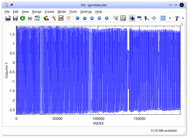
Note that no field was specified for the X axis of the plot, so Kst used the default INDEX vector. The INDEX vector is a special vector in Kst that contains integers from 0 to N-1, where N is the number of frames read in the corresponding Y axis vector. Close Kst by selecting from the menu, or by typing Ctrl+Q.
gyrodata.dat contains 20000 frames, so you may
wish to only look at a portion of the data. To only plot 10000 frames
starting from frame 7000, type:
kst2 gyrodata.dat -f 7000 -n 10000 -y 1
One of Kst's strengths is its ability to plot real-time data.
Imagine that new data was being continually added to the end of
gyrodata.dat. In such a scenario, it would be
useful to only plot the most recent portion of the data. To plot only
the last 1000 frames of gyrodata.dat, enter the
following:
kst2 gyrodata.dat -n 1000 -y 1
If gyrodata.dat was being updated, the plot would
continuously scroll to display only the last 1000 frames.
Note that the description of the y option states that
Multiple instances of the y option are allowed. This allows quick
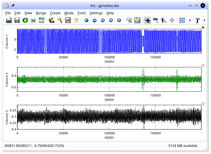
plotting of more than one curve. To plot
all three fields in gyrodata.dat in separate
plots, arranged in one column, enter the following:
kst2 gyrodata.dat -m 1 -y 1 -y 2 -y 3
The m option specifies that the plots should be in a single column.
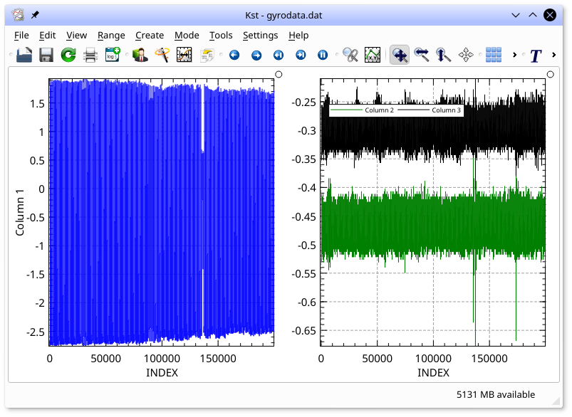
To plot column 1 in one plot, and columns 2 and three in a second plot, displayed side by side enter:
kst2 gyrodata.dat -m 2 -P 1 -y 1 -P 2 -y 2 -y 3
| Prev | Contents | Next |
| The Kst Tutorial | Up | Creating plots with the Data Wizard |