
| Plugins, Fits, and Filters |
| Prev | Next |
Table of Contents
Many of the mathematical data operators in Kst, including fits and filters, are implemented as plugins. Plugins are loaded at run time and use a stable API, so it is possible to write your own plugins and include them in your local installation without re-compiling Kst. Fits and Filters are simply subsets of the set of plugins, and thus behave identically to generic plugins, with the exception of additional convenience dialog functionality when selected from the plot context menu. See here for a general description of the creation of fits and filters.
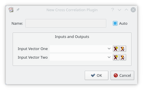
To date, there are more than 25 built-in plugins available in Kst that perform functions from taking cross correlations of two vectors to producing periodograms of a data set. The following screenshot shows the settings window for a typical plugin, created by selecting the desired plugin from the , or submenus in the toolbar menu.
The following sections describe the purpose, key algorithms or formulas used to perform calculations, and inputs and outputs for each plugin. Note that fitting and filtering plugins are included in the following sections.
The autocorrelation plugin calculates correlation values between a series (vector) and a lagged version
of itself, using lag values from floor(-(N-1)/2) to floor((N-1)/2), where N
is the number of points in the data set. The time
vector is not an input as it is assumed that the data is sampled at equal time intervals. The correlation
value r at lag k is:
The bin plugin bins elements of a single data vector into bins of a specified size. The value of each bin is the mean
of the elements belonging to the bin. For example, if the bin size is 3, and the input vector is
[9,2,7,3,4,74,5,322,444,2,1], then the outputted bins would be
[6,27,257]. Note that any elements remaining at the end of the input vector that do not form a complete
bin (in this case, elements 2 and 1), are simply discarded.
The Butterworth band-pass plugin filters a set of data by calculating the Fourier transform of the data and recalculating the the frequency responses using the following formula
where f is the frequency, fc is
the low frequency cutoff, b is the bandwidth of the band to pass, and
n is the order of the Butterworth filter. The inverse Fourier transform
is then calculated using the new filtered frequency responses.
The array of values to filter.
The order of the Butterworth filter to use.
The low cutoff frequency of the Butterworth band pass filter.
The width of the band to pass. This should be the difference between the desired high cutoff frequency and the low cutoff frequency.
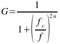
The Butterworth band-stop plugin filters a set of data by calculating the Fourier transform of the data and recalculating the the frequency responses using the following formula
where f is the frequency, fc is
the low frequency cutoff, b is the bandwidth of the band to stop, and
n is the order of the Butterworth filter. The inverse Fourier transform
is then calculated using the new filtered frequency responses.
The array of values to filter.
The order of the Butterworth filter to use.
The low cutoff frequency of the Butterworth band stop filter.
The width of the band to stop. This should be the difference between the desired high cutoff frequency and the low cutoff frequency.
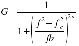
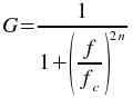
The Butterworth high-pass plugin filters a set of data by calculating the Fourier transform of the data and recalculating the the frequency responses using the following formula
where f is the frequency, fc is
the high frequency cutoff, and
n is the order of the Butterworth filter. The inverse Fourier transform
is then calculated using the new filtered frequency responses.
The array of values to filter.
The order of the Butterworth filter to use.
The cutoff frequency of the Butterworth high pass filter.
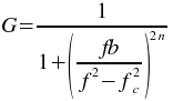
The Butterworth low-pass plugin filters a set of data by calculating the Fourier transform of the data and recalculating the the frequency responses using the following formula
where f is the frequency, fc is
the low frequency cutoff, and
n is the order of the Butterworth filter. The inverse Fourier transform
is then calculated using the new filtered frequency responses.
The array of values to filter.
The order of the Butterworth filter to use.
The cutoff frequency of the Butterworth low pass filter.
The chop plugin takes an input vector and divides it into two vectors. Every second element in the input vector is placed in one output vector, while all other elements from the input vector are placed in another output vector.
The array containing the odd part of the input array (i.e. it contains the first element of the input array).
The array containing the even part of the input array (i.e. it does not contain the first element of the input array).
The array containing the elements of the odd array minus the respective elements of the even array.
An index array the same length as the other three output arrays.
The convolution plugin generates the convolution of one vector with another. The convolution of two functions
f and g is given by:
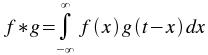
The order of the vectors does not matter, since f*g=g*f. In addition,
the vectors do not need to be of the same size,
as the plugin will automatically extrapolate the smaller vector.
One of the pair of arrays to take the convolution of.
One of the pair of arrays to take the convolution of.
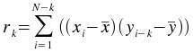
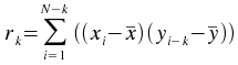
The crosscorrelation plugin calculates correlation values between two series (vectors) x and
y,
using lag values from floor(-(N-1)/2) to floor((N-1)/2), where N
is the number of elements in the longer vector. The shorter vector is padded to the length of the
longer vector using 0s. The time
vector is not an input as it is assumed that the data is sampled at equal time intervals. The correlation
value r at lag k is:
The array x used in the cross-correlation formula.
The array y used in the cross-correlation formula.
The deconvolution plugin generates the deconvolution of one vector with another. Deconvolution is the inverse of
convolution. Given the convolved vector h and another vector g, the deconvolution
f is given by:

The vectors do not need to be of the same size,
as the plugin will automatically extrapolate the shorter vector. The shorter vector is assumed to be the
response function g.
One of the pair of arrays to take the deconvolution of.
One of the pair of arrays to take the deconvolution of.
The Fit exponential weighted plugin performs a weighted non-linear least-squares fit to an exponential model:
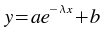
An initial estimate of
a=1.0,

=0, and
b=0 is used. The plugin subsequently iterates to the solution
until a precision of 1.0e-4 is reached or 500 iterations have been performed.
The array of x values for the data points to be fitted.
The array of y values for the data points to be fitted.
The array of weights to use for the fit.
The array of fitted y values.
The array of residuals.
The best fit parameters a,
, and
b.
The covariance matrix of the model parameters, returned row after row in the vector.
The weighted sum of squares of the residuals, divided by the degrees of freedom.
The Fit exponential plugin is identical in function to the
Fit exponential weighted
plugin with the exception that the weight value wi
is equal to 1 for all index values i. As a result, the
Weights (vector) input does not exist.
The Fit gaussian weighted plugin performs a weighted non-linear least-squares fit to a Gaussian model:
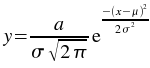
An initial estimate of
a=(maximum of the y values),

=(mean of the x values), and

=(the midpoint of the x values)
is used. The plugin subsequently iterates to the solution
until a precision of 1.0e-4 is reached or 500 iterations have been performed.
The array of x values for the data points to be fitted.
The array of y values for the data points to be fitted.
The array of weights to use for the fit.
The array of fitted y values.
The array of residuals.
The best fit parameters
,
, and
a.
The covariance matrix of the model parameters, returned row after row in the vector.
The weighted sum of squares of the residuals, divided by the degrees of freedom.
The Fit gaussian plugin is identical in function to the
Fit gaussian weighted
plugin with the exception that the weight value wi
is equal to 1 for all index values i. As a result, the
Weights (vector) input does not exist.
The gradient weighted plugin performs a weighted least-squares fit to a straight line model without a constant term:

The best-fit is found by minimizing the weighted sum of squared residuals:
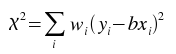
for b,
where wi is the weight at index i.
The array of x values for the data points to be fitted.
The array of y values for the data points to be fitted.
The array containing weights to be used for the fit.
The array of y values for the points representing the best-fit line.
The array of residuals, or differences between the y values of the best-fit line and the y values of the data points.
The parameter b of the best-fit.
The estimated covariance matrix, returned row after row, starting with row 0.
The corresponding value in Y Fitted minus the standard deviation of the best-fit function at the corresponding x value.
The corresponding value in Y Fitted plus the standard deviation of the best-fit function at the corresponding x value.
The value of the sum of squares of the residuals, divided by the degrees of freedom.
The Fit linear plugin is identical in function to the
Fit gradient weighted
plugin with the exception that the weight value wi
is equal to 1 for all index values i. As a result, the
Weights (vector) input does not exist.
The Fit linear weighted plugin performs a weighted least-squares fit to a straight line model:

The best-fit is found by minimizing the weighted sum of squared residuals:
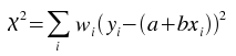
for a and b,
where wi is the weight at index i.
The array of x values for the data points to be fitted.
The array of y values for the data points to be fitted.
The array containing weights to be used for the fit.
The array of y values for the points representing the best-fit line.
The array of residuals, or differences between the y values of the best-fit line and the y values of the data points.
The parameters a and b of the best-fit.
The estimated covariance matrix, returned row after row, starting with row 0.
The corresponding value in Y Fitted minus the standard deviation of the best-fit function at the corresponding x value.
The corresponding value in Y Fitted plus the standard deviation of the best-fit function at the corresponding x value.
The value of the sum of squares of the residuals, divided by the degrees of freedom.
The Fit linear plugin is identical in function to the
Fit linear weighted
plugin with the exception that the weight value wi
is equal to 1 for all index values i. As a result, the
Weights (vector) input does not exist.
The Fit lorentzian weighted plugin performs a weighted non-linear least-squares fit to a Lorentzian model:
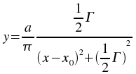
An initial estimate of
a=(maximum of the y values),
x0=(mean of the x values), and

=(the midpoint of the x values)
is used. The plugin subsequently iterates to the solution
until a precision of 1.0e-4 is reached or 500 iterations have been performed.
The array of x values for the data points to be fitted.
The array of y values for the data points to be fitted.
The array of weights to use for the fit.
The array of fitted y values.
The array of residuals.
The best fit parameters
x0,
, and
a.
The covariance matrix of the model parameters, returned row after row in the vector.
The weighted sum of squares of the residuals, divided by the degrees of freedom.
The Fit lorentzian plugin is identical in function to the
Fit lorentzian weighted
plugin with the exception that the weight value wi
is equal to 1 for all index values i. As a result, the
Weights (vector) input does not exist.
The Fit polynomial weighted plugin performs a weighted least-squares fit to a polynomial model:
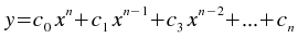
where n is the degree of the polynomial model.
The array of x values for the data points to be fitted.
The array of y values for the data points to be fitted.
The array of weights to use for the fit.
The order, or degree, of the polynomial model to use.
The array of fitted y values.
The array of residuals.
The best fit parameters c0,
c1,...,
cn.
The covariance matrix of the model parameters, returned row after row in the vector.
The weighted sum of squares of the residuals, divided by the degrees of freedom.
The Fit polynomial plugin is identical in function to the
Fit polynomial weighted
plugin with the exception that the weight value wi
is equal to 1 for all index values i. As a result, the
Weights (vector) input does not exist.
The Fit sinusoid weighted plugin performs a least-squares fit to a sinusoid model:

where T is the specified period,
and n=2+2H, where
H is the specified number of harmonics.
The array of x values for the data points to be fitted.
The array of y values for the data points to be fitted.
The array of weights to use for the fit.
The number of harmonics of the sinusoid to fit.
The period of the sinusoid to fit.
The array of fitted y values.
The array of residuals.
The best fit parameters c0,
c1,...,
cn.
The covariance matrix of the model parameters, returned row after row in the vector.
The weighted sum of squares of the residuals, divided by the degrees of freedom.
The Fit sinusoid plugin is identical in function to the
Fit sinusoid weighted
plugin with the exception that the weight value wi
is equal to 1 for all index values i. As a result, the
Weights (vector) input does not exist.
The Interpolation Akima spline plugin generates a non-rounded Akima spline interpolation for the supplied data set, using natural boundary conditions.
The array of x values of the data points to generate the interpolation for.
The array of y values of the data points to generate the interpolation for.
The array of x values for which interpolated y values are desired.
The kstinterp akima periodic plugin generates a non-rounded Akima spline interpolation for the supplied data set, using periodic boundary conditions.
The array of x values of the data points to generate the interpolation for.
The array of y values of the data points to generate the interpolation for.
The array of x values for which interpolated y values are desired.
The Interpolation cubic spline plugin generates a cubic spline interpolation for the supplied data set, using natural boundary conditions.
The array of x values of the data points to generate the interpolation for.
The array of y values of the data points to generate the interpolation for.
The array of x values for which interpolated y values are desired.
The Interpolation cubic spline periodic plugin generates a cubic spline interpolation for the supplied data set, using periodic boundary conditions.
The array of x values of the data points to generate the interpolation for.
The array of y values of the data points to generate the interpolation for.
The array of x values for which interpolated y values are desired.
The Interpolation linear plugin generates a linear interpolation for the supplied data set.
The array of x values of the data points to generate the interpolation for.
The array of y values of the data points to generate the interpolation for.
The array of x values for which interpolated y values are desired.
The Interpolation polynomial plugin generates a polynomial interpolation for the supplied data set. The number of terms in the polynomial used is equal to the number of points in the supplied data set.
The array of x values of the data points to generate the interpolation for.
The array of y values of the data points to generate the interpolation for.
The array of x values for which interpolated y values are desired.
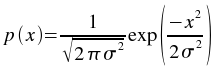
The Noise addition plugin adds a Gaussian random variable to each element of the input vector.
The Gaussian distribution used has a mean of 0 and the specified
standard deviation. The probability density function of a Gaussian random variable is:
The array of elements to which random noise is to be added.
The standard deviation to use for the Gaussian distribution.
The periodogram plugin produces the periodogram of a given data set. One of two algorithms is used depending on the size of the data set—a fast algorithm is used if there are greater than 100 data points, while a slower algorithm is used if there are less than or equal to 100 data points.
The array of time values of the data points to generate the interpolation for.
The array of data values, dependent on the time values, of the data points to generate the interpolation for.
The factor to oversample by.
The average Nyquist frequency factor.
The statistics plugin calculates statistics for a given data set. Most of the output scalars are named such that the values they represent should be apparent. Standard formulas are used to calculate the statistical values.
The mean of the data values.
The minimum value found in the data array.
The maximum value found in the data array.
The variance of the data set.
The standard deviation of the data set.
The median of the data set.
The absolute deviation of the data set.
The skewness of the data set.
The kurtosis of the data set.
| Prev | Contents | Next |
| Exporting Tabs | Up | Licensing |