Getting Started

This is a brief introductory tutorial to the fundamental features of Kst. We will cover...

Importing Data

Let's start by seeing how raw data can be imported into Kst using the graphical interface (this can also be done using the command line, for details see the appendix on Command Line Options).

Begin by running Kst. When you do this for the first time, a “QuickStart” Dialog should appear by default.

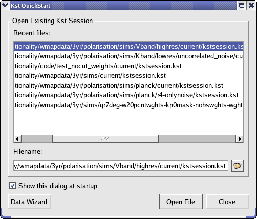
This dialog has a list of your recently opened Kst sessions, as well as a link to the Data Wizard. The Data Wizard allows data to be imported into Kst using the graphical interface. We'll run through using it now.

Click the Data Wizard button. A data source dialog will appear which allows you to select a file or network resource (e.g. HTTP address) to use as a data source. Kst determines the format of the source by its extension and contents.

We will import data from a file called “gyrodata.dat” which should be included in your Kst installation. The location of this file is $KDEDIR/share/apps/kst/tutorial/gyrodata.dat, where $KDEDIR is the location in which KDE is installed on your system (you can find this using the command kde-config --prefix).

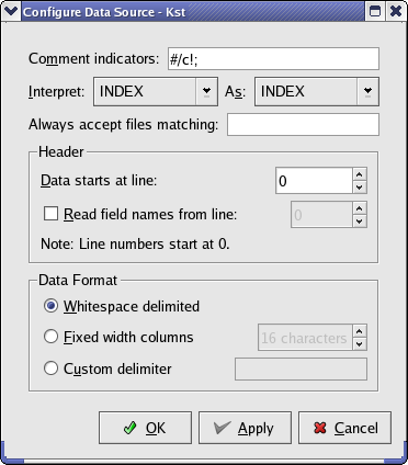
Select gyrodata.dat for opening. Kst should report the data source as type ASCII, which means that the data is in delimited plain text format. More options can be seen by clicking the Configure button. The options for the gyrodata.dat file should be as shown below:

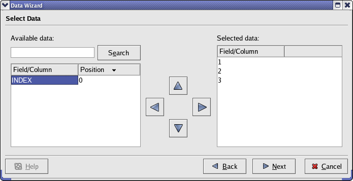
Close the Configure Data Source Dialog and click the Next button. This will lead to a pane where you can select the fields from the data source which you'd like to work with. In the case of ASCII data, each field is a column in the text file. Select the data from the 1st, 2nd, and 3rd fields. The INDEX field is a supplementary field created by Kst. It contains integers from 0 to N-1, where N is the number of frames in the data file. Once you've selected the proper fields, the selection pane should look like this:

Click the Next button again, to get to the Data Presentation Pane. This allows you to select some basic and frequently modified options for the plots which are about to be created.

The Data Range section is used to specify the subset of data to read from the selected vectors in the input file. For more information about this pane see the Data Wizard documentation.

Configure the Data Presentation Pane to look like the following:

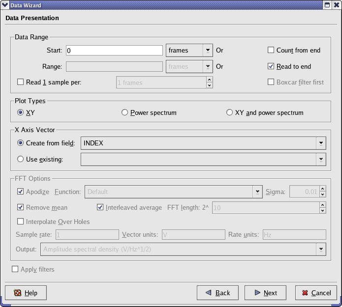
This tells Kst that we would like to read all of the available data for our chosen fields, and that we would like to generate plots with the x-axis of the data as its INDEX. INDEX is an automatically generated vector which gives the position of the data elements within the file.

Clicking the Next button again takes us to the final Data Wizard pane, where there are options to determine the appearance of the plotted data. We can select a curve style, decide whether labels and legends should be generated from the available field names, and decide which plots the curves should be placed into. Again, the default options should be fine for now.

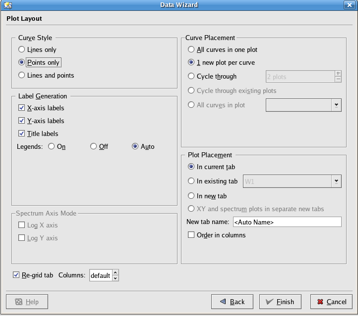
Now, click the Finish button to generate the plots. Your Kst session should now look something like this:

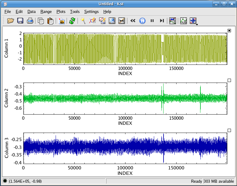
Congratulations! You've just done some basic plotting in Kst. Generating these plots took a bit of effort, so we should save the current Kst session (it will be used in the next section of this tutorial). Select Save As... from the File menu, and save the session as mykstsession.kst:

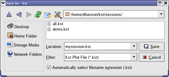
Saving the Kst session allows you to restore your plots later.

Plot Manipulation

Now that you are comfortable with creating plots from imported data in Kst, we can explore some of the plot manipulation features available through the graphical user interface. Start Kst from the command-line with the mykstsession.kst file you saved earlier:

kst mykstsession.kst

All the plots you created in the Importing Data section should now be loaded in Kst. Examine the plots with the y axis label of Column 2. To take a closer look at the plot, right click on it and select the Maximize menu item, as shown below:

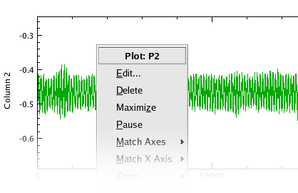
The plot you selected will now be maximized within the current window. Note that the data is still dense in this plot, so it would be useful to zoom in on an interesting area. To do so, make sure you are in XY Mouse Zoom mode (select XY Mouse Zoom from the Plots menu, or click the toolbar button). Then, simply drag a rectangle around the area you're interested in. Note that the coordinates of the mouse cursor are displayed in the lower right corner of the Kst window (if they are not, ensure that Show Statusbar is checked in the Settings menu).

The plot axes will change to “zoom in” on the selected area of the plot. Suppose that you would like to view some data just outside the region you have zoomed into. This can be done with Kst's scrolling feature. Right-click on the plot and select Up, Down, Left, or Right from the Scroll submenu. The plot will scroll accordingly. Of course, it is usually easier to use the shortcut key associated with the menu item; this is true for most of the zooming and scrolling functions. The shortcut keys for scrolling are the Arrow keys, so the quickest way to scroll upwards would be to hold down the Up Arrow key. To return to maximum zoom at any time, right-click on the plot and select Zoom Maximum from the Zoom submenu (or type M, the shortcut key associated with Zoom Maximum).

Restore the size of the plot by right-clicking it and unchecking the Maximize option.

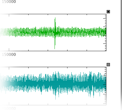
Now look at the plots with y axes labeled Column 2 and Column 3. These are plots of the pitch gyro and roll gyro, respectively, from the 1998 BOOMERANG flight. Since these two plots are related, it can be useful to zoom and scroll them simultaneously. Click on the squares located at the top right corners of the two plots. They should turn gray in color to indicate that the two plots are now tied together:

Before we try zooming in, we should delete the “Column 1” plot, which we won't be working with any more. Right-click on this plot and select Delete. A hole will be left in the plotting window. We can remedy this by right-clicking anywhere inside the window and selecting Cleanup Layout->Default Tile. Now the two remaining plots should share maximal space inside the window. Return to XY Mouse Zoom mode when you are done.

Now try zooming in on any portion of the upper plot. You will find that the lower plot becomes blank. This is because the lower plot axes have changed to match the upper plot axes, and there is no data in that particular region of the lower plot. Type M while the mouse cursor is over either plot to return to maximum zoom on both plots. Now hold down Ctrl (this is equivalent to selecting X Mouse Zoom Mode from the Plots menu or clicking the toolbar button). The mouse cursor will change shape as visual feedback. While keeping Ctrl held down, drag a rectangle in the upper plot. Note that the height of the dotted rectangle is restricted so that only the x axis will be zoomed. Now both plots will display data when zoomed in, as the y axis for either plot was not changed.

Tip

You can quickly tie or untie all the plots in the window by selecting Tied Zoom from the Plots menu or by clicking the toolbar button.

When you are finished experimenting with the zooming features, you can save the mykstsession.kst file again, with the changes which have been made.

Basic Analysis and the Data Manager

There is more to Kst than simple plotting and viewing of data. From the data wizard, you have already seen that Kst has the ability to create power spectra of data. In fact, Kst is also capable of creating other data objects such as histograms, equations, and plugins. A utility called the Data Manager can help you to do this.

Open the data manager now by clicking the toolbar button, or by selecting Data Manager from the Data menu.

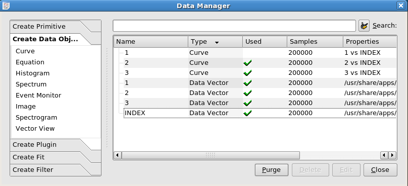
The Data Manager contains the definitive list of data objects in the current Kst session. It also allows you to edit or create new data objects. As you can see, there are currently 3 curves (each created from a pair of vectors) and four data vectors listed. A summary is given for each object; see the Data Manager section for more information.

We saw earlier that when we attempted tied-zoom in XY-Zoom-Mode that the Column 2 and Column 3 data have different y-offsets. Suppose that we would like to compare them on the same graph. To do this, we will have to shift the mean of one of the plots. We can do this easily using an Equation Object.

Begin the process of creating an Equation by clicking the corresponding button under the Create Data Object tab on the left side of the Data Manager. A dialog will appear to create the new object. Configure this dialog as shown below:

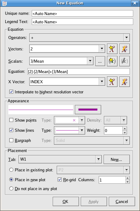
This equation takes values from the data vector [2], subtracts the scalar [2/mean], then adds the scalar [3/mean] to make a new vector which is [2] shifted vertically to have the same mean as the data vector [3]. Note from the Scalars drop-down menu that Kst maintains a collection of simple statistics on all of its vectors (as well as many other objects). These can frequently prove useful.

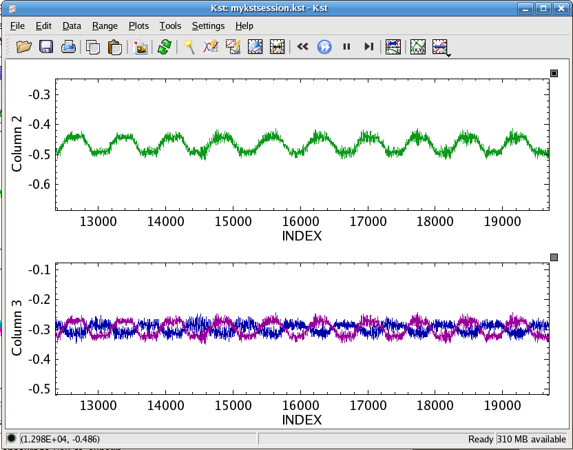
Click the OK button of the New Equation dialog. Now a new curve has been added to the plot with y-axis label “Column 3”. If we return to the Kst plot window, we can zoom in on the “Column 3” plot. Comparing the data, we can see what we suspected, that data vector [2] is essentially the same as [3], but exactly out of phase:

This concludes our basic introduction to Kst. We encourage you to experiment with the program now; there is clearly a lot of functionality in Kst which hasn't been covered in this tutorial. Most of it can be found intuitively. You may want to look at some of the entries in the Common Tasks chapter. Good luck!