
Curve Fitting
Kst also provides functions for many different types of curve fitting: linear, quadratic, sinusoidal, and more. As an example, we'll do a simple polynomial fit to the curve we plotted previously, in the Plotting Simple Graphs section.
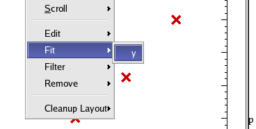
Right click on the “simple graphs” plot which you've created and select “y” from the submenu in the context menu which appears.
Now a “New Plugin” dialog will appear which allows you to configure the fit. Since the example data here are quadratic, we'll use the Fit polynomial plugin. Choose this from the Plugin Selection drop-list. As it happens, the Order of the polynomial is set to 2 by default, which is what we want. You can set the Order to any integer, one of the predefined scalar quantities, or some statistical value based on one of the available vectors (e.g. the Standard Deviation of x, [x/Sigma]).
There are several Output fields where you can enter text to be used as the unique name for the vectors and scalars generated by this fit. For more information, you can read the section on the Fit Polynomial in the Plugins chapter.
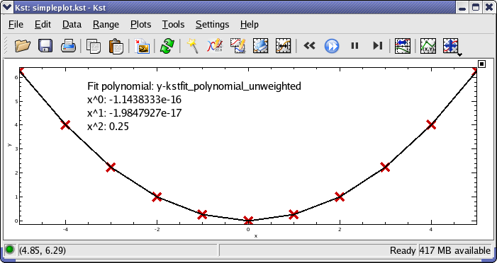
Hit to perform the fit. A new curve showing the best fit polynomial will be automatically added to the plot containing the original curve. A new label object is also added to the plot containing the fitted coefficients for x^2, x^1 and x^0 (the constant).
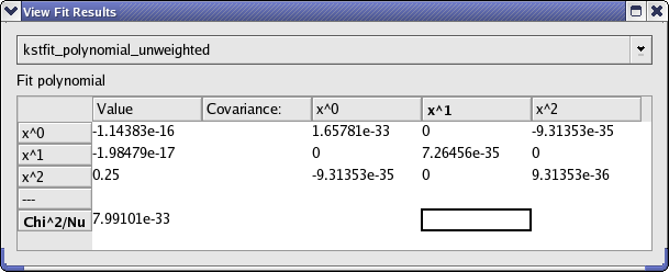
Not all of the fit results are shown in the new label. The covariances for the fit coefficients, as well as the Chi-Square value for the fit can be accessed from the View Fit Results dialog. Select -> from the main menu, and choose the fit which you are interested in from the drop down list. The results are shown in a table:


Would you like to make a comment or contribute an update to this page?
Send feedback to the KDE Docs Team